JAPANESE / ENGLISH
JAPANESE / ENGLISH
Last updated on 05/7/2021
Theoretically speaking, an optical fiber with a circular core has no birefringence, and the polarization state in such an optical fiber does not change during propagation. In reality, however, a small amount of birefringence is always present in an optical fiber due to external perturbations (load, bend, etc…) or manufacturing imperfection. Such birefringence is inherently random, and thus causes random power coupling between two polarization modes (polarization crosstalk) in an optical fiber. The output polarization state, therefore, becomes unpredictable and also varies with time.
A Polarization-Maintaining Fiber (PM Fiber, PMF) maintains two polarization modes by intentionally inducing uniform birefringence along the entire fiber length, thereby prohibiting random power coupling between two polarization modes. Examples of PMFs are schematically shown in Figure 1. Larger birefringence better prohibits the power coupling, and thus is one of the key characteristics for a PMF. A PMF is also called a birefringent fiber.
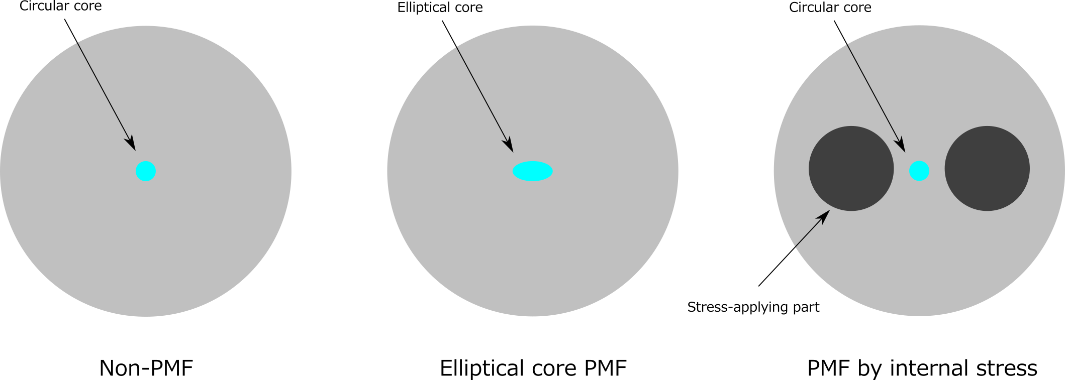
Figure 1: Schematic of PMFs. (Non PMF is also shown for comparison.)
Birefringence can be induced by introducing twofold (or less) rotational symmetry, either in the refractive-index profile or in the stress distribution. The former is called form birefringence and the latter is stress birefringence. PMFs are an essential device for guiding polarized light, and various types of PMFs are used for optical communication, fiber lasers, and fiber sensors, etc .
NOTE: This article only deals with a linearly birefringent PMF, in which two linear (i.e. x- and y-) polarization states are maintained. This is the most common form of PMF, and it is well accepted to call this type of fiber simply a PMF.
Form birefringence originates from a vector electromagnetic effect in optical fibers possessing twofold (or less) rotational symmetry . The simplest way to introduce twofold rotational symmetry in the refractive-index profile is making the shape of the core elliptical . An example of elliptical core fiber is shown in Figure 2.
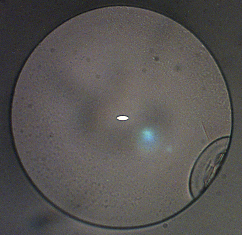
Figure 2: Cross section of elliptical core PMF. (FiberLabs ZSF-2.2×5.5/125-N-PM ZBLAN fluoride fiber)
Stress birefringence in optical fibers is thermally induced . Figure 3 schematically shows an example of PMF based on stress birefringence, most commonly known as PANDA(*) fiber or Bow-Tie fiber . The fiber has two stress-applying parts which are positioned on both sides of the core and have a thermal expansion coefficient different from the rest of the fiber. The stress-applying parts change volume at a different rate compared to the other part of the fiber when the fiber cools down to the room temperature after fiber drawing; this induces a large stress into the core of the fiber.
(*) “PANDA” stands for Polarization-maintaining AND Absorption reducing, and also is named after its similarity to panda bear.
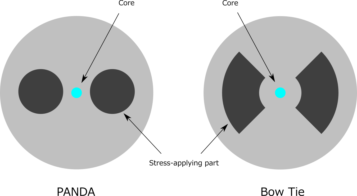
Figure 3: Schematic of PANDA and Bow-Tie fiber.
The difference in propagation constants Δβ between the two polarization modes is called modal birefringence (Bm); modal birefringence is usually normalized such that it has no unit, and provided as:
\(\displaystyle \mathrm{B_m} = \displaystyle{\frac{\Delta\beta}{k_0}} \),
where k0=2π/λ0 (λ0: wavelength in vacuum). Large modal birefringence reduces polarization crosstalk, thus enables better ability to maintain polarization modes. PMFs typically exhibit modal birefringence larger than 10-4.
Two polarization modes have different propagation constants in a PMF. Beat length (LB) is the length where the accumulated phase difference reaches 2π, and is provided as:
\(\displaystyle \mathrm{L_B (m)} = \left( \displaystyle{\frac{2π}{Δβ}} \right) = \left( \displaystyle{\frac{\lambda_0}{\mathrm{B_m}}} \right) \).
Beat length is another way to quantify the amount of birefringence, and is inversely proportional to birefringence. The larger the birefringence becomes, the shorter the beat length becomes.
There are two polarization modes in a PMF; one polarized along the x-axis and the other polarized along the y-axis. The propagation constants of these two modes are different, and the polarization direction of a mode with the larger propagation constant is called the slow axis, as the phase velocity of the mode is slower than the other. And the polarization direction of a mode with the smaller propagation constant is called the fast axis. Figure 4 shows the slow axis and fast axis of an elliptical-core fiber and PANDA fiber.
The polarization mode polarized along the slow axis is usually more well confined and robust against external perturbations; and thus is more often used.
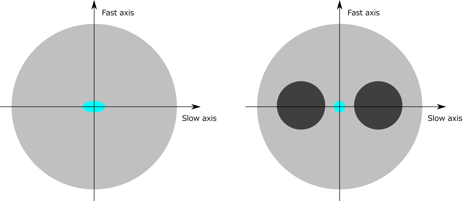
Figure 4: Slow axis and fast axis of elliptical-core and PANDA fiber.
\(\displaystyle \mathrm{Crosstalk (dB)} = \log_{10} \left( \displaystyle{\frac{P_1}{P_0}} \right) \),
where P0 is the power of the main polarization mode (at the output), and P1 is the power of the unwanted polarization mode produced by polarization crosstalk.
Figure 5: Schematic of polarization crosstalk measurement.